IT & Engineering
Machine learning for everyday tasks

Machine learning is often thought to be too complicated for everyday development tasks. We often associate it with things like big data, data mining, data science, and artificial intelligence. Sometimes it feels something like this:

Machine Learning is hard
I have always felt like we can benefit from using machine learning for simple tasks that we do regularly.
Real life example
At Mailgun, we work with e-mail and as part of our offering, we parse HTML quotations. This allows a user to grab the latest reply instead of the entire conversation, which is returned as part of our webhook response. You can read more about how we handle inbound message processing in our documentation.
For those of you who don’t know, here’s what parsing HTML from the public Internet looks like:

Parsing HTML from public internet
It’s messy and sometimes processes get stuck.
Changing the parsing library can help, but it won’t solve the issue completely because every library has its limitations. You have to restrict the parsing to something reasonable.
Cluster analysis to the rescue
But what should the criteria and threshold be? Should we limit by HTML length or tag count? Maybe both? Maybe by something else? The objective obviously is to process as many messages as possible without shooting yourself in the foot, but the path isn’t super obvious.
That’s where cluster analysis and statistical classification become handy. For the research I was using R, but depending on your task and personal preferences you might use something else – scikit-learn, Weka, MOA, etc.
Collect a dataset
First, we logged HTML length, tags count, message processing time and put them into a csv file:
htmllen,tagscount,took rn2893762,85527,34.300139904 rn31378,518,0.0368919372559 rn19105,413,0.0545339584351 rn...
The vast majority of messages take fractions of a second to process. So, when collecting the dataset, we had to make sure that we have enough “slow” messages.
We ended up with two csv files, collected on different days. One had 13831 lines and was reserved for analysis and model-training (the train dataset). Another had 12149 lines and was reserved for model validation (the validation dataset).
Generally you want to have at least two datasets – one for training and one for validation. Otherwise you might run into overfitting problem, when your model is well adjusted to the train data but fails in the real world.
Determine the number of clusters
To visualize the data and look for patterns k-means clustering was first tried:
messages <- read.csv(file="messages080816.csv", sep=",", head=TRUE) rn mydata <- matrix(messages$took, ncol=1) rnrn ## Determine the number of clusters rn wss <- (nrow(mydata)-1)*sum(apply(mydata,2,var)) rn for (i in 2:15) wss[i] <- sum(kmeans(mydata, rn centers=i)$withinss) rn plot(1:15, wss, type="b", xlab="Number of Clusters", rn ylab="Within groups sum of squares")
As you can see there is a significant performance improvement up to 4 clusters. After that there is no real boost.
Clustering
The next step was to figure out how the data points get distributed between the clusters:
## K-Means Clustering with 4 clustersrn fit <- kmeans(mydata, 4) rnrn ## Cluster Plot against 1st 2 principal components rn ## vary parameters for most readable graph rn library(cluster) rn clusplot(mydata, fit$cluster, color=TRUE,rn shade=TRUE, labels=2, lines=0)
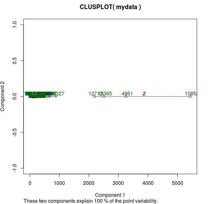
And you can somewhat anticipate the problem already: the clusters form by nipping off the datapoints that are far away, while the interval we’re interested in (1-20 sec) is in the very midst. The issue persists with increasing the number of clusters.
Moreover there is a significant overlap between the clusters in the interval:
## get clusters mean, min, max rn mean <- aggregate(mydata,by=list(fit$cluster),FUN=mean) rn min <- aggregate(mydata,by=list(fit$cluster),FUN=min) rn max <- aggregate(mydata,by=list(fit$cluster),FUN=max)
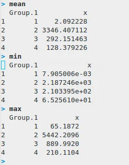
Compare clusters number 1 and 4. The issue persists with increasing the number of clusters.
At this point, we decided to try a different approach and look at the percentiles for message processing time:
percentiles <- quantile(messages$took, seq(0.5, 0.99, 0.01)) rn plot(seq(0.5, 0.99, 0.01), percentile)
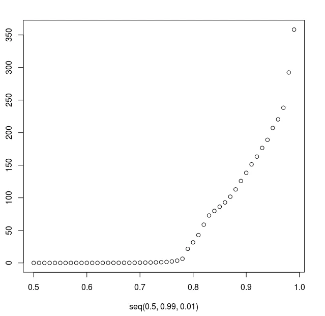
As you can see, after the 78th percentile the processing time quickly bubbles up. Here was our first threshold – 78th percentile that corresponded to 6.5 seconds.
All datapoints that took less than 6.5 sec were marked as “fast” and others as “slow”.
Classification
For classification, we tried SVM (Support Vector Machines), Random Forests and CART(Classification And Regression Tree).
CART showed slightly better results for this task but its main advantage is that it gives you a decision tree that is easy to understand, explain and implement vs SVM or Random Forests that work like a black box and require using heavy ML libraries in production.
Here’s how you classify using CART:
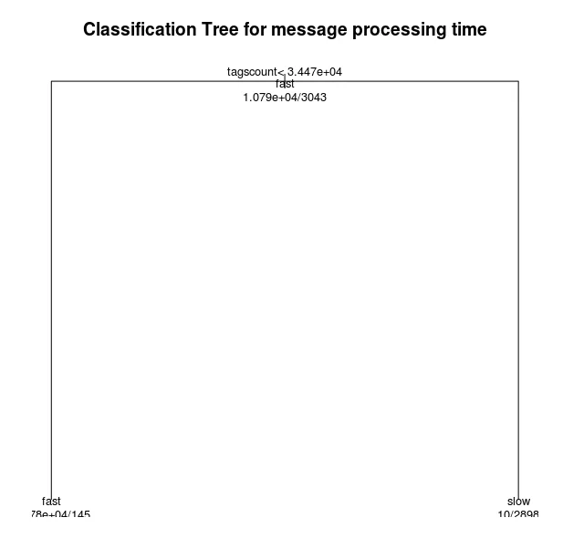
x <- subset(messages, select=-took) rnlibrary(rpart) rnrn# grow tree rnfit <- rpart(x$cls ~., method="class", data=x) rnrn## display the results rnprintcp(fit)rnrn# detailed summary of splits rnsummary(fit) rnrn# plot tree rnplot(fit, uniform=TRUE, rn main="Classification Tree for message processing time") rntext(fit, use.n=TRUE, all=TRUE, cex=.8)
Here’s the decision tree:
And that’s how the implementation looks like:
def html_too_big(s): rn return s.count('<') > _MAX_TAGS_COUNT
Isn’t it beautiful? All the research complexity in a single line!
Validation
For evaluation we took the validation dataset and tried to predict the classification using our model:
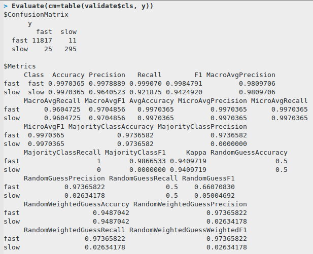
validate <- read.csv(file="messages080916.csv", sep=",", head=TRUE) rn validate <- subset(validate, select=-took) rn xv <- subset(validate, select=-cls) rn y <- predict(fit, xv, type="class") rn table(validate$cls, y)
Here’s the confusion matrix and some common classification metrics:
Lessons Learned
Machine learning is not just for data scientists. Even simple decisions powered by ML can benefit you. Know your data. Do not rely blindly on scientific algorithms and models.
Useful links
- Great explanation of a train-validate-test workflow
- Quick guide on CART and Random Forests in R
- Quick guide on Cluster Analysis in R
- How to plot in R
- Some common classification metrics
- Precision and Recall explained
Happy machine learning and data mining!