What toasters and distributed systems might have in common
A few months ago we released automatic IP Warm Up, but we never got to talk about how it’s implemented. Today, we’re going to peek under the hood and try to understand what makes our IP warm up tick. We’re going to start with some context, and then we’ll dive into the interesting technical details later in the post.
A few months ago we released automatic IP Warm Up, but we never got to talk about how it’s implemented. Today, we’re going to peek under the hood and try to understand what makes our IP warm up tick. We’re going to start with some context, and then we’ll dive into the interesting technical details later in the post.
Let’s face it — no one likes receiving tons of information all at once. The same can be said for mailbox providers receiving your emails. Spammers usually blast out their campaigns over a short period of time, so the providers don’t like that behavior. To protect themselves from abuse, they’ll block messages that come from an IP that has never sent an email before. Some providers might still accept the messages, but those messages will go right to spam. That’s not good for anybody.
To get those messages into the inbox we better start delivering fewer of them and ramp up the volume over time to build up a reputation; that’s why it is called “warm up.” Think about warming up a car engine before flooring it or doing light exercises before lifting weights at a gym, it’s a bit like that.
When you sign up for a Mailgun account, you get a shared IP. A shared IP means it’s used by multiple customers, so it’s already warmed up and has a good reputation. You don’t have to worry about it unless another sender causes its reputation to go down. Now you want to add a dedicated IP, and we’ve talked about why you might want that as your sending volume grows. The dedicated IP that you get is fresh and has no reputation, hence mailbox providers know nothing about it. We don’t pre-warm them because we want your IP to be tied to what you’re sending and so you can build your own reputation over time. That will lead to better results. Does it mean you still have to send only a few messages from the start? Yes, we know that it’s not ideal.
That’s where automatic IP warm up comes in. When a dedicated IP gets added, the shared IP still remains on your account, so we can divert the traffic to it during the warm-up. Over time, we can increase the volume a little bit at a time to send more and more messages until the dedicated IP is fully warmed up and you’re ready to go.
A very important thing to remember, however, is that the warm-up process will not buy you great deliverability! The practices you incorporate as a sender is what drives deliverability so make sure you are taking responsibility for the messages you send out and the recipients that receive them. Otherwise, you’re just slowly deteriorating the IP reputation instead of instantly burning it!
Warm Up Plan
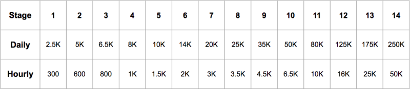
We’ve found that mailbox providers typically care about both hourly and daily volumes. Each day the volume could be increased by a few percent. This is very handy because this compound effect leads to exponential growth and the ability to ramp up in a relatively small amount of steps. We call these steps “stages”. Stages make up a “warm-up plan”, that looks like this:
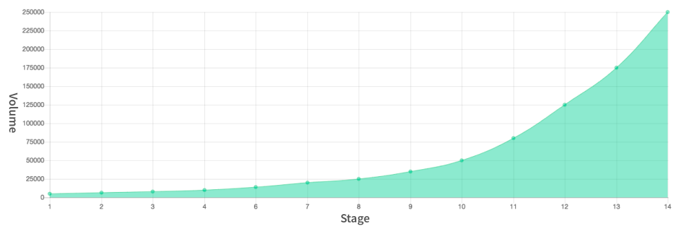
If we plot the daily amounts, we’ll get the following picture:
It consists of 14 stages and at each stage, we send a certain amount of messages from a dedicated IP. That volume was carefully determined by our deliverability team through research and is periodically updated when we collect new evidence. It turned out that sending a proper amount of messages is an interesting engineering problem and we’d like to share some details on the way we solved it.
How to maintain a certain volume
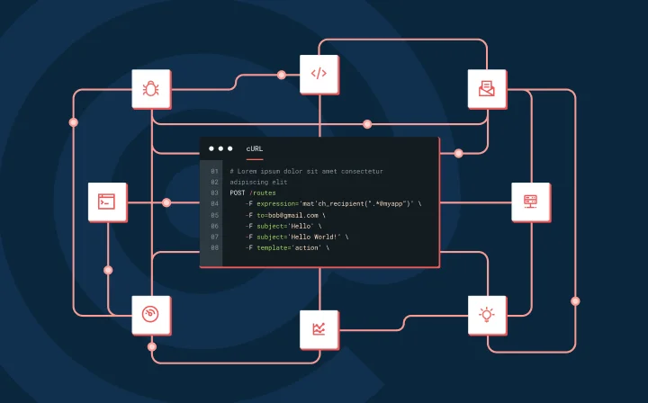
Let’s dive in and take a closer look at the implementation of an algorithm that allows us to send a given amount of messages. Now that we have a shared and a dedicated IP together, we should think about how to balance the traffic between the two of them. The easiest way to do that is to implement a random load-balancing algorithm. Imagine that we flip a coin to determine which IP a message is sent from, with the shared IP being “heads” and the dedicated IP being “tails.” If we wanted to decrease the number of messages coming from the dedicated IP, we would change the probability of getting “tails” as our outcome. This would make our coin unfair, but it works to our advantage. Here is how that might look in golang:
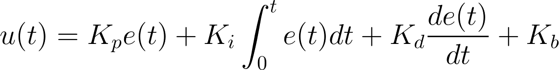
The probabilityOfDedicated can take any float value from 0 to 1.0. When it’s 1.0 all messages go through the dedicated IP and when it’s 0 everything goes through the shared one. Setting it to 0.5 will give us equal odds of sending it via the dedicated IP or shared IP. It’s essentially a knob that controls the sending flow. Let’s see how we can maintain a rate of 350 messages an hour from the dedicated IP by updating that value. The simplest thing that comes to mind is setting the probabilityOfDedicated to 1 and once the 350 message mark is reached, reset it to 0. It’s a little abrupt, but should do the trick.
const cap = 350rnfunc getProbabilityOfDedicated(sentMessages int) float64 {rn if sentMessages u003c cap {rn return 1rn }rn return 0rn}
Is it really that simple?
When we want to run a program on hundreds of servers processing hundreds of thousands of requests per second we can’t expect everything to be always updated in real-time. Optimization techniques such as batch processing and caching become our best friends. They’re great at what they were designed for, but they inevitably add a lag between a value being calculated, updated, and shared across all the nodes in a cluster. Let’s call that lag inertia from here on out.
Speaking of our example, there are many things that contribute to inertia. First, the statistics updates might not be truly real-time due to optimizations in the message counting service. Second, there is a lag between when our value of probability of picking dedicated IP gets calculated and distributed due to caching. By the time we see that a 350th message has been sent and it’s time to stop, more might slip through before the update takes an effect.
This is a working example, so feel free to paste it to go playground and play with it:
package mainrnrnimport (rn u0022fmtu0022rn u0022math/randu0022rn u0022syncu0022rn u0022timeu0022rn)rnrnvar (rn mutex = u0026sync.Mutex{}rn rnd = rand.New(rand.NewSource(99))rn messagesSent = 0 // keep track of the messages that IP sendsrn probability = 0.0 // probability of picking a dedicated IPrn)rnrnconst (rn sampleRateMsec = 50.0 // how often the system is being refreshedrn cap = 350.0 // this is how many messages we want to sendrn)rnrn// deliverySimulator will emulate the message sending process.rn// It will pick the dedicated IP based on the probability.rnfunc deliverySimulator() {rn for {rn mutex.Lock()rn if rnd.Float64() u003c probability {rn // We don't know how fast the messages arern // being submitted, let's throw somern // randomness in there to make it unpredictable.rn messagesSent += rnd.Intn(10)rn } else {rn // Shared IP will be picked here.rn }rn mutex.Unlock()rn time.Sleep(time.Millisecond)rn }rn}rnrnfunc calcProbabilityOfDedicated(sent int) float64 {rn if sent u003c cap {rn return 1rn }rn return 0rn}rnrnfunc main() {rn go deliverySimulator()rnrn // Control loop.rn for i := 0; i u003c 8; i++ {rn mutex.Lock()rnrn // Get messages.rn sent := messagesSentrnrn // Calculate probability.rn probability = calcProbabilityOfDedicated(sent)rnrn fmt.Println(u0022sent:u0022, sent, u0022probability:u0022, probability)rn mutex.Unlock()rnrn time.Sleep(time.Duration(sampleRateMsec) * time.Millisecond)rn }rn}
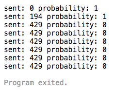
Here is the output we get:
Oops, looks like we sent many more messages than we wanted; almost 25% more as a matter of fact. What can we do about it? Well, we can come up with a threshold to stop it in advance, but that would have to be different for every customer as they all submit messages at different rates.
What if we can embrace inertia? What if we could gradually slow down?
Physical systems
Inertia is so common in the physical world. In order to control mechanical systems, engineers have to always take inertia into account. Can we learn anything from them?
The first attempts of creating an automatic controller for physical systems date back to 17th century with the centrifugal governor. It was an essential part of any steam engine at the time. Fast forward to the early 20th century where the theory behind Proportional Integral Derivative (PID) controller was developed after observing how helmsmen control ships by taking into account different environmental and system factors. These days PID controllers are used everywhere from quadcopters to toasters, and it’s because they are very simple and effective. Of course, there are many other control algorithms, but most of them are not as nearly as elegant.
A little bit of Control Theory
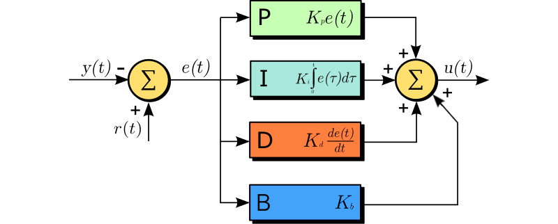
Let’s talk about the theory behind PID controllers. For starters, they only work when there is a feedback loop. Feedback loops are pretty straightforward in that the result of the control action gets piped back to the controller input. It’s like an ouroboros if the mythology symbolism helps, and if not, there’s this diagram.
Let’s take a closer look at the controller block and open it up.
Whoa, that’s a lot. It’s a little overwhelming so let’s break it down a bit. First, we need to agree on terminology. Here are a few terms to be familiar with going in:
Process variable – y(t), the current value of the thing we want to control. In our case, it would be the number of messages sent from an IP and will serve as the feedback.
Setpoint – r(t), the value we want to land at. In our example, it’s the cap of 350 messages.
Error – e(t), the current difference between a setpoint and a process variable. e(t) = r(t) – y(t).
Control variable – u(t), the output of the controller, this will drive our probability of picking a dedicated IP.
All variables are written as a function f(t), which means its value changes in relation to time t, so it’s a value at that very moment of time. The diagram can be described by the classic formula from any textbook on the control theory:
There are 4 terms in this equation — proportional + integral + derivative + bias. Each of them contribute to the control signal and the weight of their contributions can be set by respective coefficients: Kp, Ki, Kd and Kb.
Proportional term (block P of diagram 2) is the most important term of the equation. As the name states, it’s proportional to the error. The bigger the error, the bigger control force will be applied to the system.
Integral term (block I of diagram 2) is useful for getting to the setpoint faster. It accumulates the errors over time and tries to help the proportional term to correct for them. It has a very important drawback for our use case though — potential overshoot. The nature of the integral term is that it’s slow to kick in at the beginning, but when enough error is accumulated over time it can put the system in overdrive getting past the setpoint. In the most extreme case, it can lead to what is called integral windup.
Derivative term (block D of diagram 2) is proportional to the rate of change. As we reduce the error, the derivative term actually becomes negative. We can think of it as if we approach the setpoint too fast it, it will slow us down. Usually, it results to a more gradual change of the process variable.
Bias term (block B of diagram 2) is just a constant; it’s not used often but might be useful to still drive the value when it’s close to the setpoint. At that point, the error is small and the proportional term is not that pronounced.
Think about these terms as if they were all in a panel of judges voting on the decision of what the next step should be. The controller acts based on the scores they give. Since they have different personalities they all score a bit differently. The proportional is the most reasonable judge and always gives a higher score the further we are from the setpoint. The integral gets impatient if we’re not reducing the error for too long so it scores higher as time goes on. The derivative is always nervous and scores negatively if the error is reduced too fast. The bias always scores the same no matter what.
Applying the theory to our problem
Now that we’re familiar with the theory, let’s apply it. We can use the existing control loop from the previous example. One of the hardest thing implementing this is to pick proper control coefficients. Tuning the PID process is not straightforward, and there are few techniques out there that can help us with that. However, we’ve found that the fastest way is to create a simulation script and play with the parameters. They might not be perfect, but they will be good enough to solve the problem.
Here is how we might think of the coefficients in regards to our problem.
Proportional will decrease the probability of picking a dedicated IP the closer we are to the desired cap. So, when we start, the term value is big and it goes down to 0 as we send more and more messages.
Integral is tricky and we might not even need it, as we can’t correct the overshoot. The messages can’t be deleted once they are sent out.
Derivative is a very important one. It will help us to correct for the situation when the messages are submitted too fast. When that happens the term becomes big enough and starts counteracting other terms. Since it is negative when that happens it will reduce the probability and, in turn, reduce the amount of messages that get sent out from a dedicated IP.
Bias might be very useful if we’re not planning to rely on the integral term. When we get really close to the desired cap the proportional term will be small and it won’t be able to drive the value toward it as hard. This is when bias could give it a little kick.
Now that we know all of that we can replace calcProbabilityOfDedicated with the following code:
const (rn // These coefficients has been picked by trial-and-error.rn Kp = 0.42 // proportional coefficientrn Ki = 0.000001 // can be removed to simplify the algorn Kd = 1.2 // derivative coefficientrn Kb = 0.1 // fairly small in this examplern)rnrnvar (rn errorVal = 0.0rn prevError = 0.0rn integral = 0.0rn)rnrnfunc calcProbabilityOfDedicated(sent int) float64 {rn prevError = errorValrnrn // Calculate terms.rn errorVal = cap - float64(sent)rn integral = integral + (errorVal * float64(sampleRateMsec))rn derivative := (errorVal - prevError) / float64(sampleRateMsec)rnrn // Calculate PID control responsern probability := Kp*errorVal + Ki*integral + Kd*derivative + Kbrnrn // With given parameters the output is roughly within [0: 100]rn // Let's shape it to [0: 1]rn probability /= 100rn if probability u003e 1 {rn return 1rn }rn if probability u003c 0 {rn return 0rn }rnrn return probabilityrn}
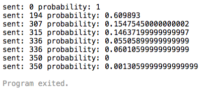
So we get this:
As you can see it works like a charm. We quickly ramped up to 300, slowed down and eventually got to 350, then the probability went down close to 0 naturally. How cool is that?!
Results
In reality, the algorithm might not set the value precisely, but it has one major advantage — it can easily be distributed. Imagine if one of the workers picks up and locks an IP, calculates the probability, saves it, and then off to the next one. This allows us to control the volume of thousands of IPs simultaneously.
Now that we have that figured out, we can create a warm up plan. It would consist of stages, where each stage has a maximum amount of messages assigned to it. As we progress through the stages this maximum volume increases and you are free to send out more and more messages. This gives you the ability to send as fast as you’re used to from a shared IP, while we gradually warm up a fresh dedicated one.
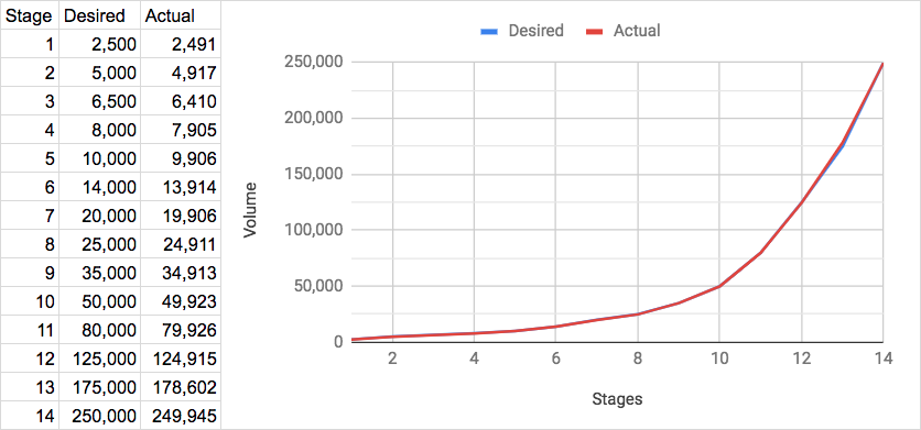
Let’s see how it works in production. Here we plotted the volume at each stage. The desired values come from the plan and actual are what was sent out.
Looks good! Before rolling it out we created a simulation environment that allowed us to test different scenarios. This is how we managed to get the values for the coefficients lined up. To our big surprise, it worked out when we deployed it to production the first time… oh, if only it happened for every deployment!
Most people would agree cookies make life better. For us, they help us make our site and marketing better. But if you don’t like cookies, that’s cool – you can let us know by clicking the settings button!
Your Cookie Choices
When you visit any web site, it may store or retrieve information on your browser, mostly in the form of cookies. This information might be about you, your preferences or your device and is mostly used to make the site work as you expect it to. The information does not usually directly identify you, but it can give you a more personalised web experience. Because we respect your right to privacy, you can choose not to allow some types of cookies. Click on the different category headings to find out more and change our default settings. However, blocking some types of cookies may impact your experience of the site and the services we are able to offer. Cookie Statement
These cookies are necessary for the website to function and cannot be switched off in our systems. They are usually only set in response to actions made by you which amount to a request for services, such as setting your privacy preferences, logging in or filling in forms. You can set your browser to block or alert you about these cookies, but some parts of the site will not then work. These cookies do not store any personally identifiable information.
Cookie details
These cookies allow us to count visits and traffic sources so we can measure and improve the performance of our site. They help us to know which pages are the most and least popular and see how visitors move around the site. All information these cookies collect is aggregated and therefore anonymous. If you do not allow these cookies we will not know when you have visited our site, and will not be able to monitor its performance.
Cookie details
These cookies enable the website to provide enhanced functionality and personalisation. They may be set by us or by third party providers whose services we have added to our pages. If you do not allow these cookies then some or all of these services may not function properly.
Cookie details
These cookies may be set through our site by our advertising partners. They may be used by those companies to build a profile of your interests and show you relevant adverts on other sites. They do not store directly personal information, but are based on uniquely identifying your browser and internet device. If you do not allow these cookies, you will experience less targeted advertising.
Cookie details
These cookies are set by a range of social media services that we have added to the site to enable you to share our content with your friends and networks. They are capable of tracking your browser across other sites and building up a profile of your interests. This may impact the content and messages you see on other websites you visit. If you do not allow these cookies you may not be able to use or see these sharing tools.
Cookie details